

How To Add Markers In Excel
For the purpose of amend information visualization, we could hands add a marker line. To highlight unlike types of important information, a marker line is a very wise choice. If you are curious to learn how to add a mark line in an Excel graph, this commodity may come up in handy for you. In this article, nosotros are going to discuss, how you tin can add together a mark line in Excel with elaborate explanations.
Download Practice Workbook
Download this practise workbook below.
3 Suitable Examples to Add together a Marker Line in Excel Graph
Adding a mark line could literally make the data visualization easier. We will use the IF, MAX, and Boilerplate functions to create those marker lines.
Example 1: Add Marker Line in Line Chart
Using a helper column, we can add together a marking line in the line chart. Nosotros will also use the IF and the MAX functions.
Steps
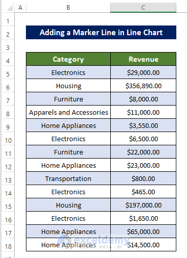
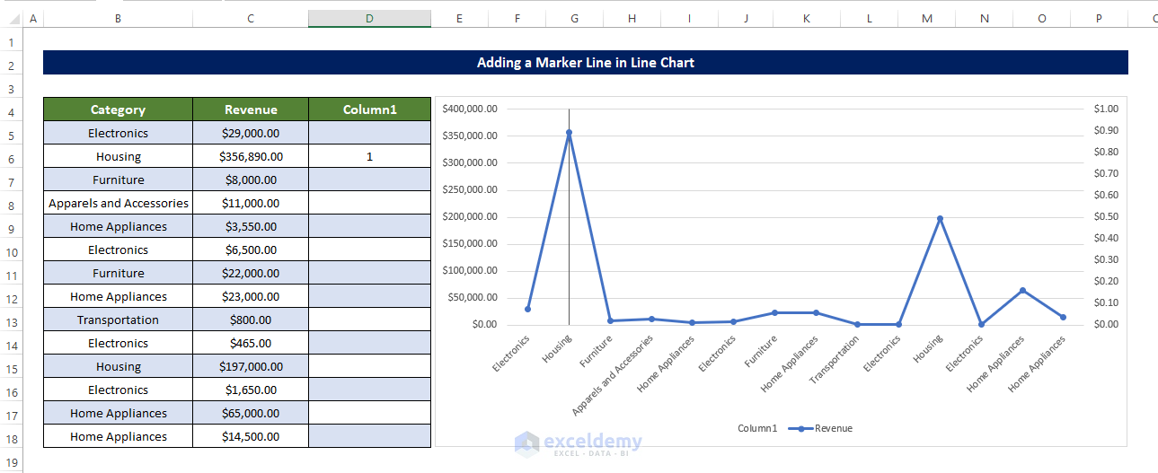
- We have the information in which we are going to add the marker in the line chart.
- Select cell D5 and enter the post-obit formula:
=IF(MAX($C$5:$C$18)=$C5,1,"")
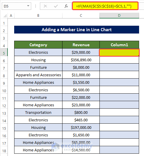
- Then drag the Fill Handle to cell D18.
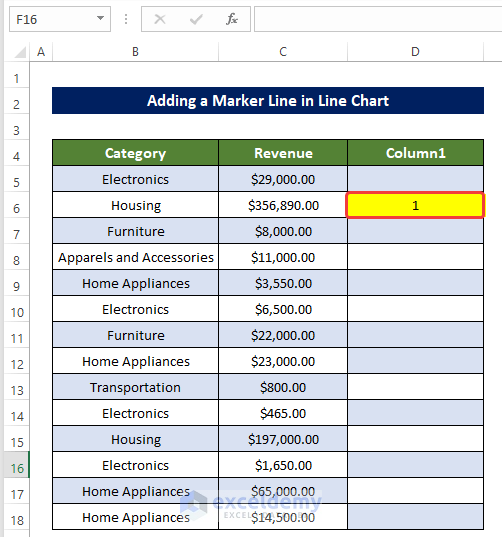
- Doing this will search for the maximum value and compare each cell value with the maximum value.
- After that, it will put ane on the side of the maximum value.
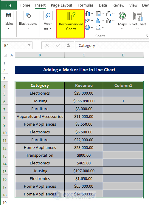
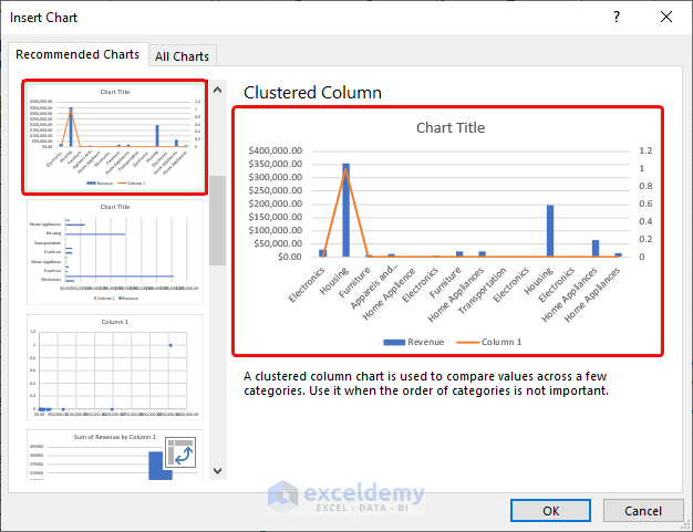
- And so select the whole data range B4:D18 and and then go to Insert Tab > Charts group.
- From in that location, click on the Recommended Charts.
- Afterward that, a new window volition open. In that window, select the Clustered Column chart as shown in the image below.
- Click OK afterwards this.
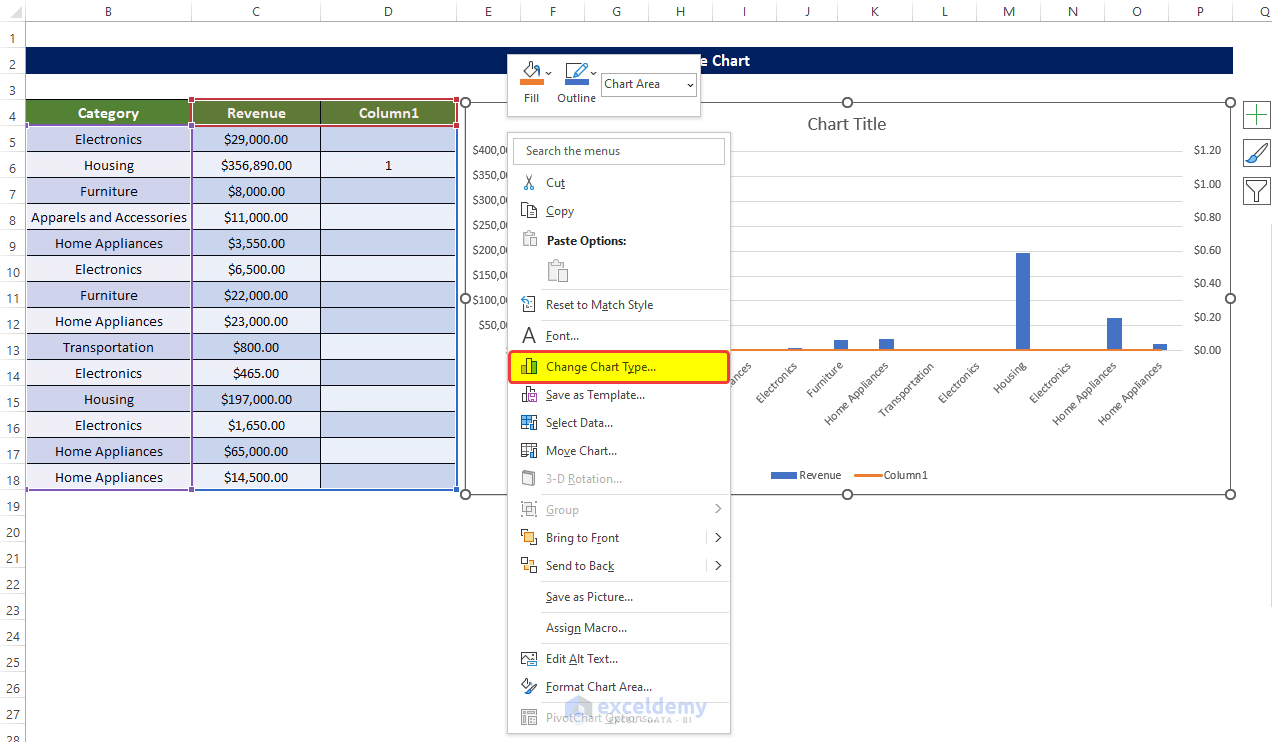
- Yous will see a new nautical chart with both the Columns (Acquirement) and Line (Column 1) nowadays.
- Right-click on the chart and select Modify Chart Type.
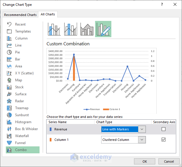
- Another new window will open and from that window, select the Chart Type for the Revenue as Line with Markers.
- And ready chart blazon for Column one as Clustered Cavalcade.
- Click OK afterwards this.
- Then you volition find that the chart is at present modified according to our settings.
- At present correct- click on the rightmost centrality.
- And from the context menu, click on the Format Axis.
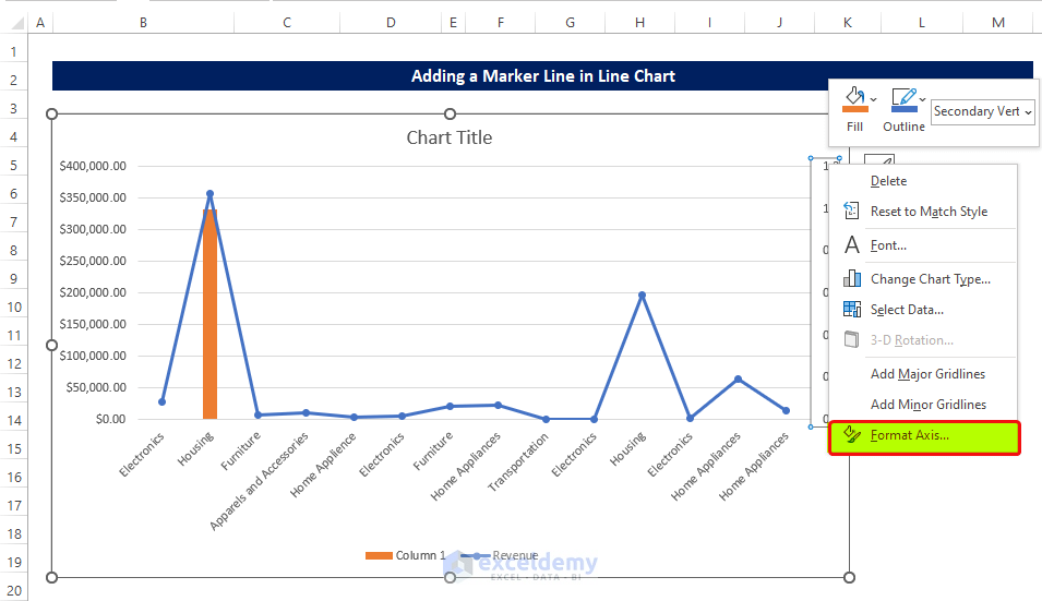
- In the Format Centrality side panel, go to the Centrality Options and then set the Maximum value every bit ane.
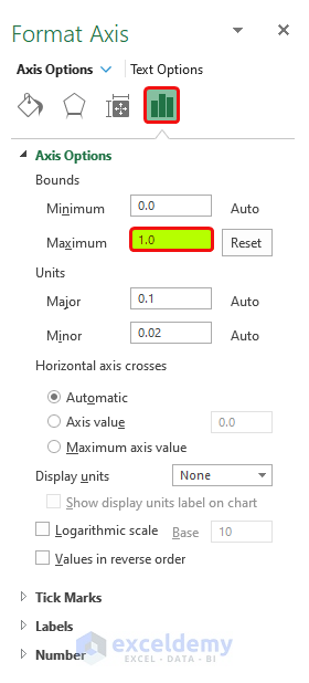
- After setting the Max value to 1, we will see that the cavalcade is at present touched the ceiling of the chart.
- Next, click on the plus sign on the side of the chart and then Fault Confined > More Options.
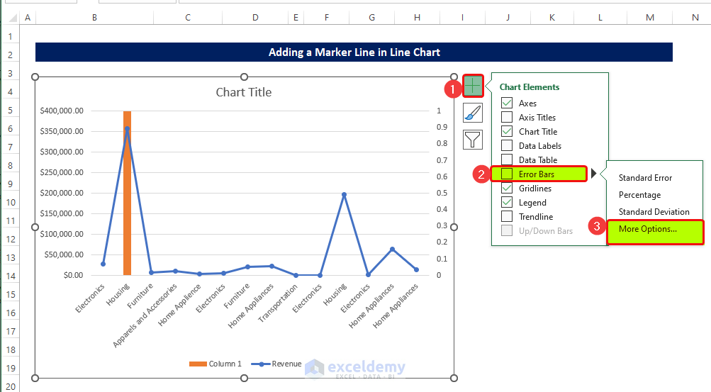
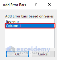
- After clicking the More than Options, nosotros will meet a new dialog box named Add Error Bar.
- From that window, click on Column ane and then click OK.
- A new side panel volition open on the right side of the sheet.
- From that panel, select Minus from the Vertical Error Bar.
- And fix the per centum to 100% in the Mistake Amount.
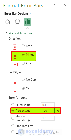
- The chart is now having a vertical line to the top of the ceiling.
- Now select the column, and right-click on it.
- From the context menu, click on the Format Data Serial.
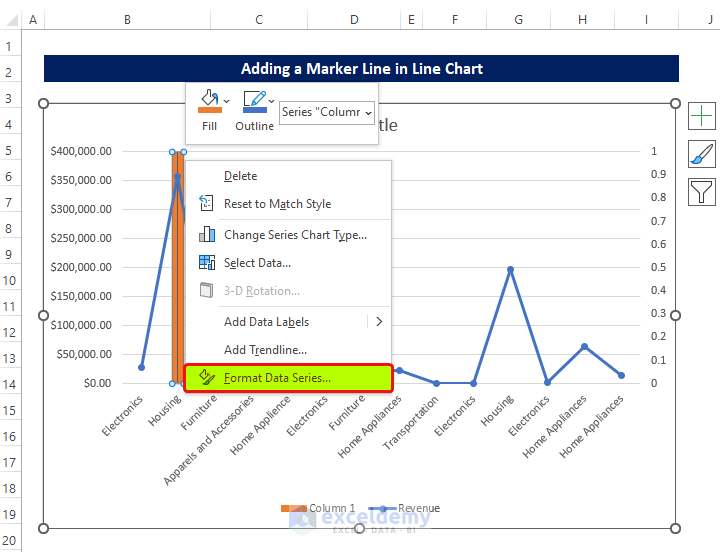
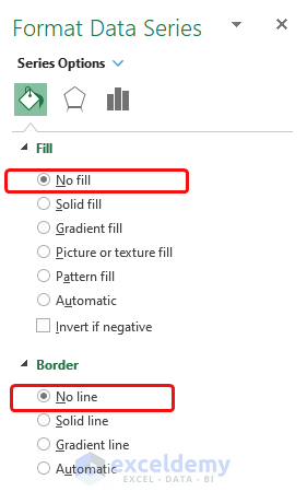
- In the side panel, select No Fill in the Fill Options.
- And No Line in the Border options.
- Finally, you volition see the marker line added for the maximum value in your Excel graph.
Read More: How to Add a Marker Line in Excel Graph (3 Suitable Examples)
Like Readings
- Make a Double Line Graph in Excel (iii Like shooting fish in a barrel Means)
- How to Combine Bar and Line Graph in Excel (two Suitable Means)
- Depict Target Line in Excel Graph (with Easy Steps)
- How to Draw a Horizontal Line in Excel Graph (2 Piece of cake Ways)
- Make a Single Line Graph in Excel (A Short Way)
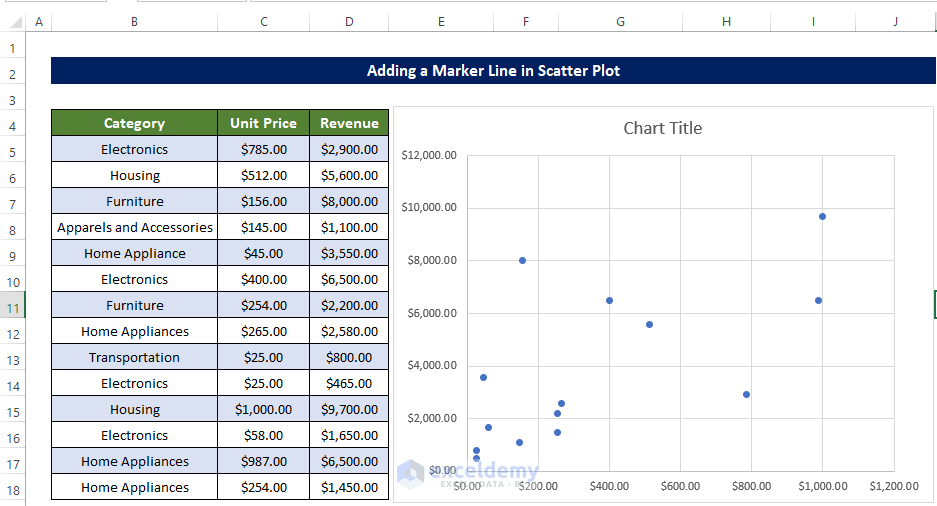
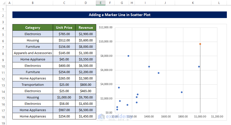
Example 2: Add together Marking Line in Besprinkle Plot
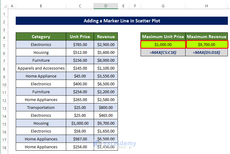
We can plot the maximum value of datasets and marking them using mistake bars. We will use the MAX part to approximate the maximum value.
Steps
- In the commencement, select the range of cells B5:D18, and then create a besprinkle plot out of it.
- The scatter plot volition await like the below prototype.
- Now select cell G5 and enter the following formula:
- Then select cell H5 and enter the following formula:
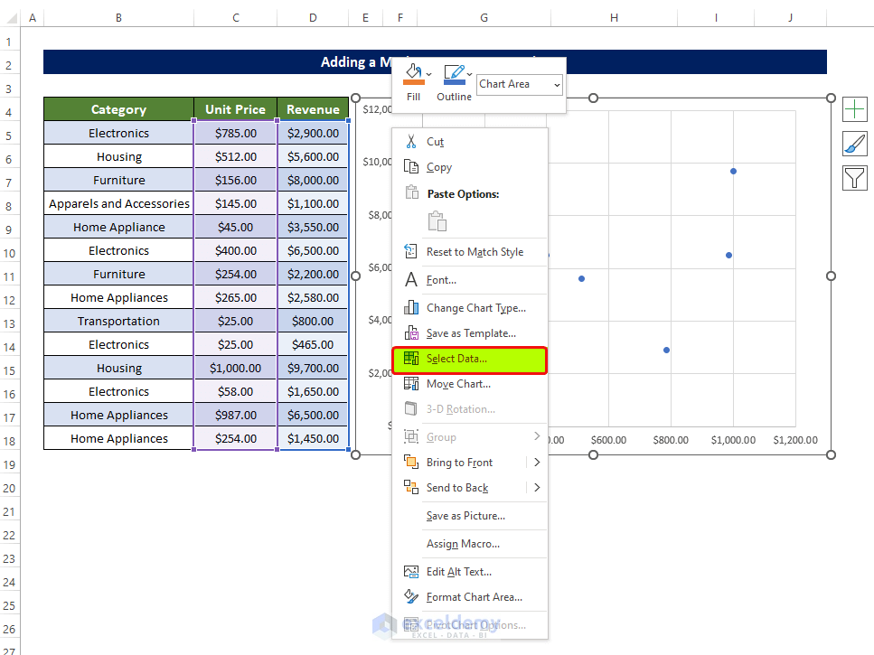
- Then right-click on the chart and from the context carte du jour, click on Select Data.
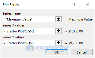
- And then select the jail cell G5 in the Series X values.
- And select prison cell H5 in the Serial Y values.
- Click OK after this.
- After this, you will see the data point is now showing in the chart. In orangish colour.
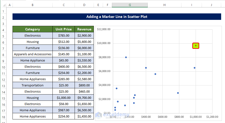
- Select the newly added information betoken and click on the Plus Sign.
- Then go to Fault bars > Percentage.
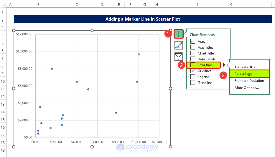
- Two mistake confined, one in the vertical direction and another one in the horizontal management are shown on the information betoken.
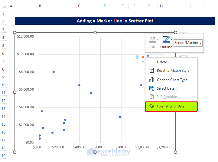
- Click on the Horizontal Error bar and then right-click on it.
- From the context carte du jour, click on the Format Fault Bar.
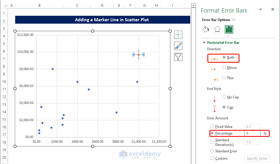
- In that location will be a new side panel named Format Error Bar. From that console, select Both in the Management options.
- And fix the Percentage to 0% in the Error Amount.
- And then select the Vertical Error bar without endmost the side panel.
- Select Minus in the Management option.
- And set the Percentage to 100% in the Fault Amount.
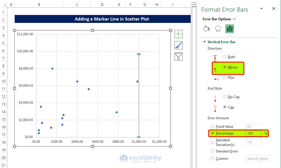
- Subsequently then, yous volition see the marker line in the nautical chart which marks the Maximum values of both the Unit of measurement Price values and the Revenues.
Read More: How to Brand a Line Graph in Excel with Multiple Lines (4 Like shooting fish in a barrel Ways)
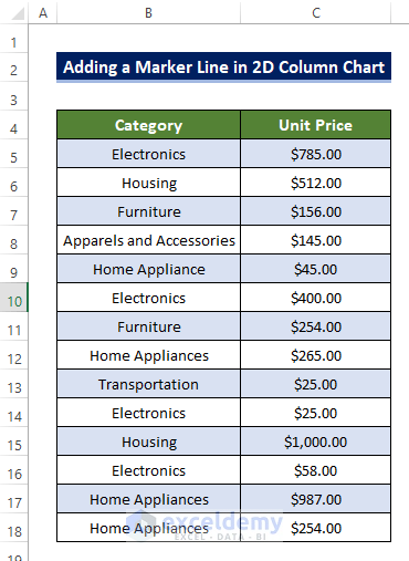
Example 3: Add Marker Line in 2D Cavalcade Chart
We can approximate the average of a range of data and marking it in a 2nd cavalcade chart with the help of the errors bar. Nosotros will utilize the Boilerplate function to attain this.
Steps
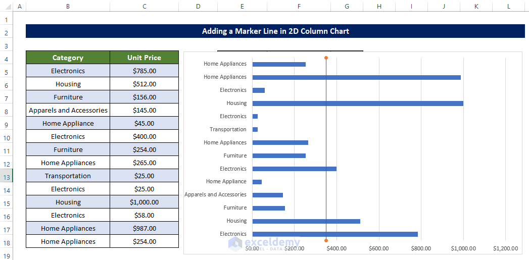
- We need to mark the average value of the products listed here in the chart.
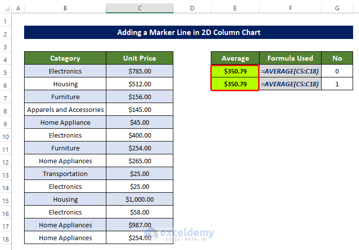
- To exercise this, first select cell E5 and enter the following formula:
- Repeat the same process for cell E6.
- And input 0 in jail cell G5 and input 1 in cell G6.
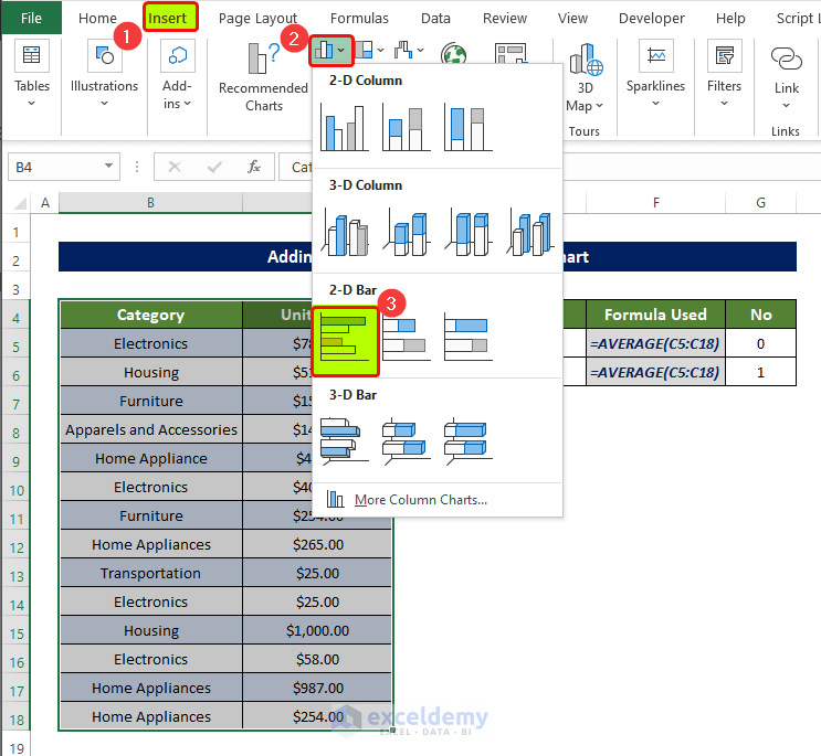
- Then select the range of cells B4:C18, and then go to Insert tab > Charts group.
- From there click on the ii-D Bar.
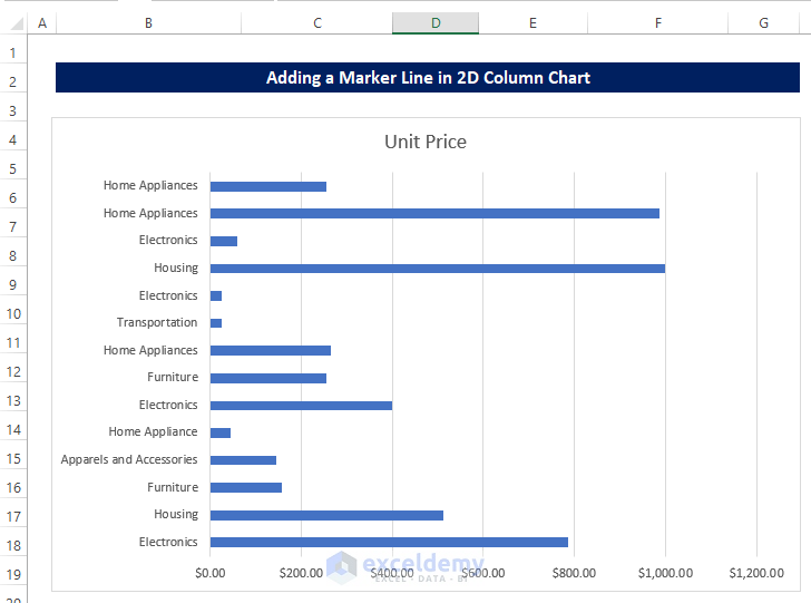
- Then you will notice that there is a ii-D bar chart near the toll of products.
- After selecting the ii-D nautical chart, we will see that there is a chart demonstrating the price of the products.
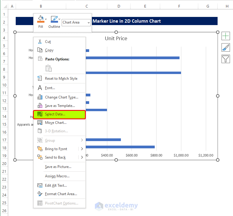
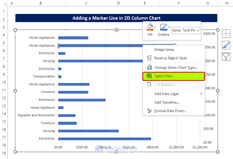
- Select the chart and right-click on it.
- From the context carte, click on Select Data.
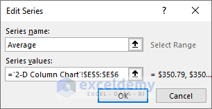
- Then click on the Add together Button in the post-obit dialog box.
- Then in the Edit Series dialog box, select E5:E6 in the Serial Values range box.
- Click OK later on this.
- And so you will see the Average value in the chart.
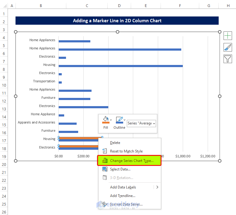
- Select the average data bar and right-click on it.
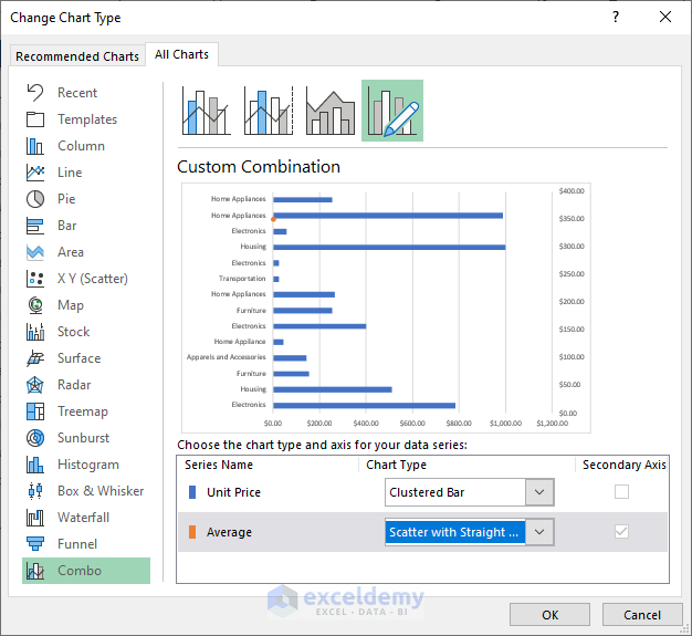
- From the context menu, click on the Change Serial Nautical chart Type.
- Then in the modify nautical chart type window, select Clustered Bar in the Unit Cost.
- And and then select Scatter with Straight Line in the Average.
- Click OK after this.
- So select the dataset and correct-click on it.
- From the context menu, click on Select Data.
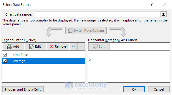
- There will be a new dialog box named Select Data Source.
- On that box, click on the previously created Average.
- And then click on Edit.
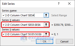
- Then on the Edit Series dialog box, select E5:E6 in the Series X values.
- And then select G5:G6 in the Series Y values.
- Click OK after this.
- After clicking ok, you volition see that there is an orange line marking the Average of the Products Unit of measurement Prices showing.
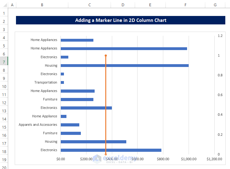
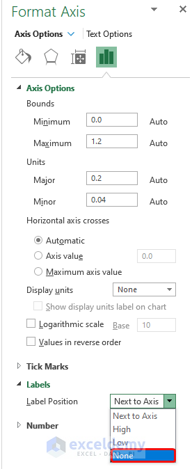
- Correct-click on the axis and from the side panel, click on the labels
- And then from the position of the label, select None from the driblet-down carte.
- After some modifications, we got the marker line that will denote the Average value of the Production prices.
Read More: How to Brand Line Graph in Excel with 2 Variables (With Quick Steps)
Conclusion
Here, we created 3 different types of marker line improver examples in the 2D chart, Scatter plot, Line nautical chart, etc. We generally marked Average values and Maximum values.
For this problem, a workbook is bachelor for download where y'all tin practice these methods.
Feel gratuitous to inquire any questions or feedback through the comment department. Whatever suggestion for the edification of the Exceldemy community volition be highly appreciable.
Related Articles
- How to Make a Line Graph in Excel with 2 Sets of Data
- Make a 100 Pct Stacked Bar Chart in Excel (with Easy Steps)
- How to Brand Legend Markers Bigger in Excel (iii Easy Means)
- Add Markers for Each Month in Excel (With Easy Steps)
- How to Brand Line Graph with 3 Variables in Excel (with Detailed Steps)
- Overlay Line Graphs in Excel (3 Suitable Examples)
- How to Brand a Line Graph in Excel with Multiple Variables
- Add a Vertical Dotted Line in Excel Graph (3 Easy Methods)
Source: https://www.exceldemy.com/add-a-marker-line-in-excel-graph/
0 Response to "How To Add Markers In Excel"
Post a Comment